Understanding the Math behind Vision Transformers(ViT)
What is a Vision Transformer?
Inspired by the Transformer scaling successes in Natural Language Processing (NLP), the experiments with applying transformers directly to images with few possible modifications resulted in the paper called Vision Transformers(ViT), which was introduced in the paper "An Image is Worth 16x16 Words". Before ViT, the dominant approach for vision was CNNs (Convolutional Neural Networks), which process images using local sliding filters.
Transformer expects a sequence, not a 2D grid. So they chopped the image into patches (e.g. 16×16 pixels each) and flattened them into vectors. To understand the difference:
| NLP Transformers | ViT |
|---|---|
| Sentence | Image |
| Word | Patch |
Transformers treat every patch equally and have no built-in notion that nearby patches are more related than distant ones. It has to learn all of this from data. So, It is also important to know that ViT loses to ResNet on standard ImageNet (~1.2M images) without any strong regularisation. However, the picture changes if the models are trained on larger datasets (14M–300M images), which trumps inductive bias.
What is an Inductive Bias? (Analogy)
Imagine you're teaching two students to recognise cats. You show them only 10 cat photos.
Student A is told beforehand:
"Cats look the same regardless of where they are in the photo"
"Focus on small local features — ears, whiskers, eyes"
Student B is told nothing. They have to figure out everything from scratch.
After 10 photos, Student A wins easily. Not because they're smarter, but because they started with useful assumptions that happen to be true about images.
Those pre-loaded assumptions = inductive bias.
CNN has a strong inductive bias, whereas the transformer has no inductive bias and must learn everything from the data.
Vision Transformer Architecture
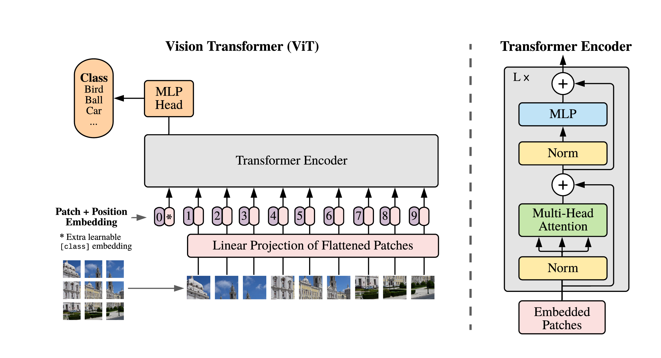
Figure 1: Vision Transformer Architecture
Patch + Positional Embedding Step-by-Step Understanding
Image to Patch:
Before a Vision Transformer can process an image, it faces one fundamental problem: Transformers expect a sequence, but images are 2D grids. The solution is surprisingly simple: cut the image into small patches and treat each patch like a word.
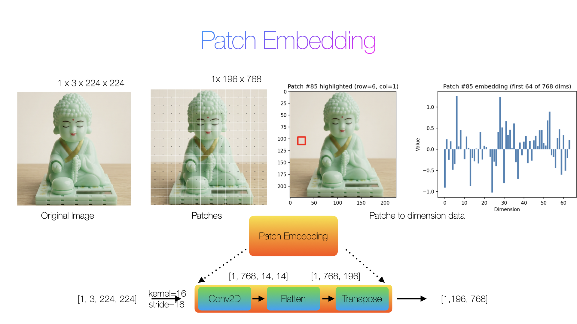
Figure 2: Patch Embedding on Buddha
Input: As shown in Figure 2, the input is a 224×224×3 image of Buddha.
Convolution: A convolution process occurs with a Kernel Size of 16 and a Stride of 16. This splits the image into a 14×14 grid of patches and maps each patch to a 768-dim vector. The output is still spatially arranged (height = 14, width = 14).
Flattern: Collapses dimensions from index 2 onward: the 14×14 grid becomes a flat list of 196 positions. Now it's [Batch size, embed_dim, N_patches].
Transpose: Swaps the embed_dim and N_patches axes to get [B, N_patches, embed_dim]. This is the standard sequence format a transformer expects: a batch of sequences, where each token is a 768-dim vector.
The number 768 is not random; it comes from a specific design decision in the original paper for the base variant (ViT-Base) as shown in Figure 3. But why 768, why not 700 or 800? Two reasons for this:
a. The authors deliberately aligned ViT-Base's dimensions with BERT-Base from NLP (which also uses D=768, 12 layers, 12 heads)
b. The Transformer splits the embedding across multiple attention heads. ViT-Base uses 12 heads, so: 768/12 = 64
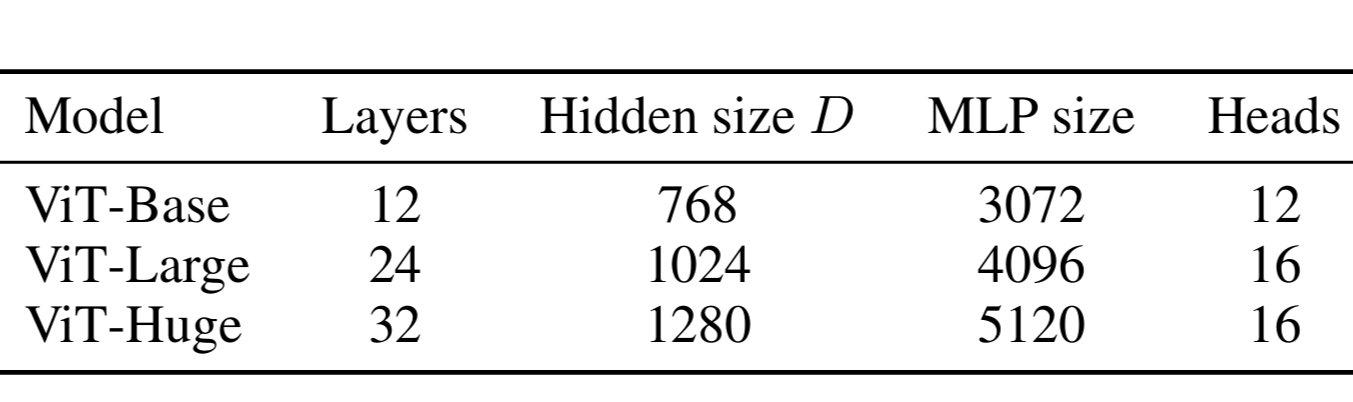
Figure3: ViT model Variants
This is the output of the features look for a single patch. I have just plotted for first 64 dimensions out of 768
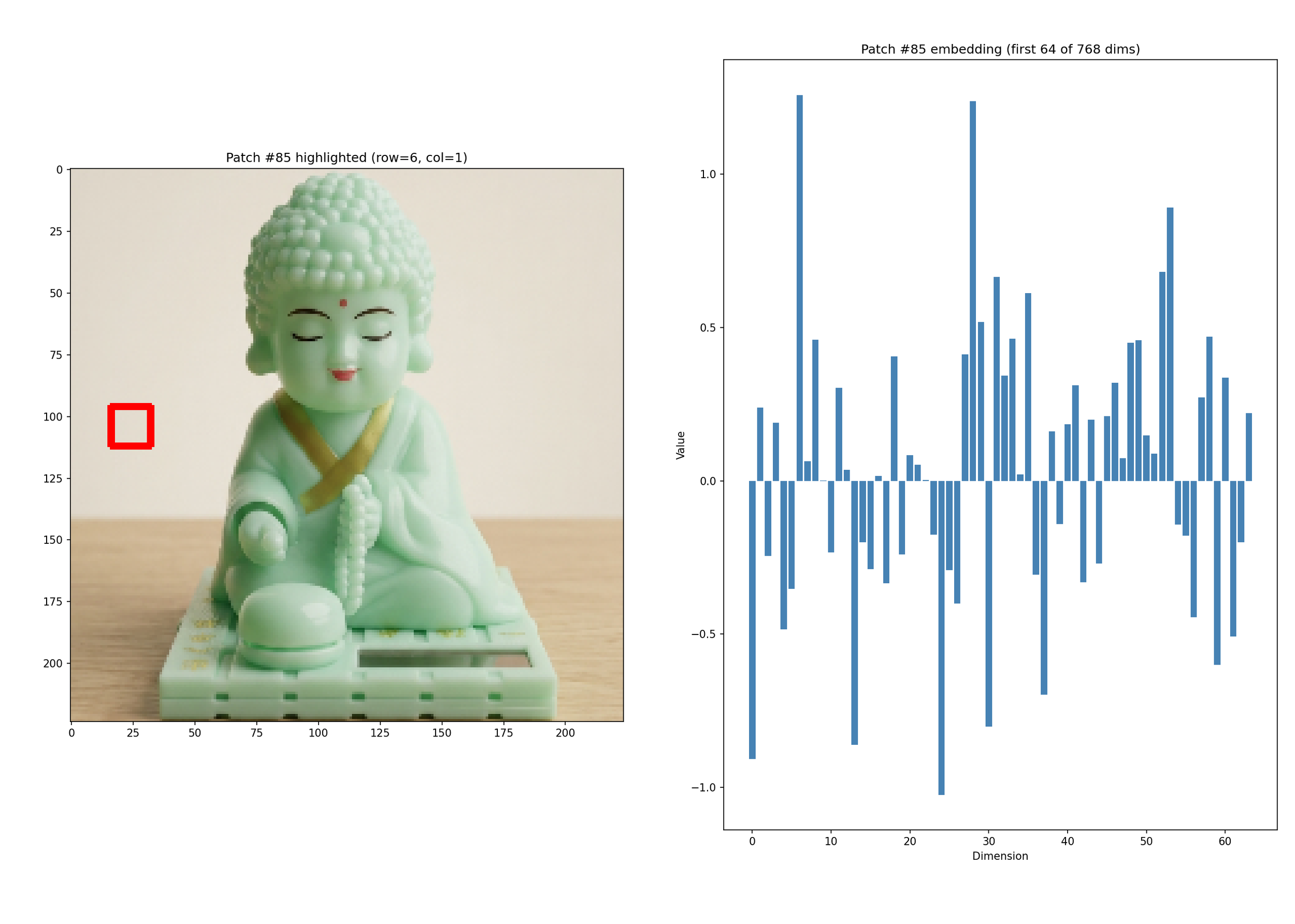
Figure4: Single patch visualization
Summary of patch embedding:
  [B, 3, 224, 224]
        ↓  Conv2d (kernel=16, stride=16)
  [B, 768, 14, 14]
        ↓  flatten(2)
  [B, 768, 196]
        ↓  transpose(1,2)
  [B, 196, 768]   ← 196 patch tokens, each with 768 features

What output  represents:
[B, 196, 768]
 ↑   ↑    ↑
 │   │    └── each patch is described by 768 numbers (features)
 │   └─────── there are 196 patches (the sequence)
 └─────────── B images in the batch

Patch #0   → [f1, f2, f3, f4, ..., f768]   ← 768 numbers describing top-left patch
Patch #1   → [f1, f2, f3, f4, ..., f768]
Patch #2   → [f1, f2, f3, f4, ..., f768]
...
Patch #195 → [f1, f2, f3, f4, ..., f768]   ← 768 numbers describing bottom-right patch
Global Summary Token (CLS):
The authors borrowed a trick from BERT in NLP. Prepend a special learnable token to the sequence — called the [CLS] token (classification token).
This CLS token:
Is a learnable vector of size D=768
It has no corresponding image region; it is not a patch from anywhere
Sits at position 0 in the sequence
Later, you will see how, during training, through self-attention, the CLS token attends to all 196 patches and aggregates information from the entire image into itself. By the end of the Transformer, the CLS token's output vector has "seen" and summarised every patch.
Before CLS:   [patch_1, patch_2, ..., patch_196]   → 196 tokens
After CLS:    [CLS, patch_1, patch_2, ..., patch_196]   → 197 tokens
Positional Embedding
After patch embedding, we have 197 tokens, with one CLS token and 196 patch tokens, each a vector of 768 numbers. But there is a fundamental problem. The Transformer has no idea where any patch came from. Shuffle all 196 patches randomly, and the Transformer sees exactly the same thing. A patch from the top-left corner and a patch from the bottom-right corner are completely indistinguishable. There is no built-in sense of order, position, or spatial layout. This is a direct consequence of how self-attention works every token attends to every other token equally, with no notion of distance or proximity built in.
The solution is to add a unique vector to each token that encodes its position.
One learnable vector of 768 numbers for each of the 197 positions — 1 for CLS and 196 for patches. These vectors start as random noise and are updated during training exactly like any other weight in the network. The most common misconception is thinking positional embeddings are just indices, That is the concept “yes”. But a Transformer cannot work with raw integers. Every token must be a vector of the same size (768 dimensions). So each position index gets its own unique 768-dimensional vector instead.
patch_1 content  : [ 0.82,  0.44, -0.31,  0.67, ...]   768 numbers from pixels
position_1 embed : [-0.14,  0.07,  0.91, -0.22, ...]   768 learned numbers
                  +
----------------------------------------------------------------------------------
result           : [ 0.68,  0.51,  0.60,  0.45, ...]   768 numbers — both fused
In the Figure 5, we add random init positional embedding with the original patch content, then we will get a positional embedding for the original images. (For visualization only fewer dimensions are visualized)
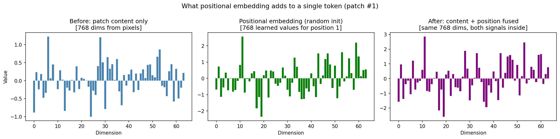
Figure 5: Adding positional embedding to patch content
How does the Input looks like before it goes to the Transformer Encoder Block? As shown in Figure 6, the first panel is the pure image content, what the Buddha image looks like after patch embedding and CLS prepend, before any position information. Notice the rows look very similar to each other; the model cannot distinguish patch #1 from patch #196 yet. Regarding the values, patch embeddings after Conv2d projection tend to produce small negative values (depends on random weight initialisation). In panel 2, mixed red and blue noise, more balanced, larger range (±4). This is what gets added: pure random noise right now. However, these are the 151,296 (197 patch x 768 dimensions) numbers that will be shaped by training into a spatial map. The final result is the positional embedding when the content and positional embedding are fused. Now this becomes the input to the Transformer Encoder block. This entire process until now is what described in the original paper as a equation, as shown in Figure7.

Figure6 : Positional Embedding
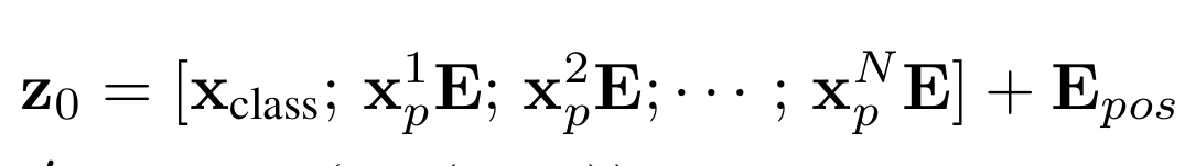
Figure7 : Equation
Patch embedding      x_p E        [B, 196, 768]
CLS token            x_class      [B, 197, 768]
Positional embedding E_pos        [B, 197, 768]
Transformer Encoder
Layer Normalisation:
During the training, as the values pass through the layers, they can become very large or very small. This is called internal covariate shift. When values explode or vanish:
gradients become unstable
learning slows down dramatically
model fails to converge
Layer Normalisation fixes this by rescaling the values before each operation.
Input to layer:    [0.5,  0.3,  0.8,  0.2]   ← reasonable values
After 4 layers:    [823,  0.001, -445, 0.0003] ← exploded/vanished
To normalize we have to do the following computation:
Compute the Mean for the 768 dimensions
Also need to compute the variance
Normalize
Finally, scale and shift using learnable parameters.
Let us apply Layer Norm manually on the CLS token after positional embedding, for explaination I have taken only 6 dimensions out of 768:
x = [-0.4828, -2.9331, -1.0430,  0.5191,  1.1593,  0.8887]

# Step 1 — Compute mean:
mu = (-0.4828 + -2.9331 + -1.0430 + 0.5191 + 1.1593 + 0.8887) / 6
   = -1.8918 / 6
   = -0.3153

# Step 2 — Compute variance:
(x0 - mu)^2 = (-0.4828 - (-0.3153))^2 = (-0.1675)^2 = 0.0281
(x1 - mu)^2 = (-2.9331 - (-0.3153))^2 = (-2.6178)^2 = 6.8529
(x2 - mu)^2 = (-1.0430 - (-0.3153))^2 = (-0.7277)^2 = 0.5295
(x3 - mu)^2 = ( 0.5191 - (-0.3153))^2 = ( 0.8344)^2 = 0.6962
(x4 - mu)^2 = ( 1.1593 - (-0.3153))^2 = ( 1.4746)^2 = 2.1744
(x5 - mu)^2 = ( 0.8887 - (-0.3153))^2 = ( 1.2040)^2 = 1.4496

var = (0.0281 + 6.8529 + 0.5295 + 0.6962 + 2.1744 + 1.4496) / 6
    = 11.7307 / 6
    = 1.9551

# Step 3 — normalize:
std = sqrt(1.9551 + 1e-5) = 1.3982

x_hat:
dim 0: (-0.4828 - (-0.3153)) / 1.3982 = -0.1675 / 1.3982 = -0.1198
dim 1: (-2.9331 - (-0.3153)) / 1.3982 = -2.6178 / 1.3982 = -1.8722
dim 2: (-1.0430 - (-0.3153)) / 1.3982 = -0.7277 / 1.3982 = -0.5205
dim 3: ( 0.5191 - (-0.3153)) / 1.3982 =  0.8344 / 1.3982 =  0.5967
dim 4: ( 1.1593 - (-0.3153)) / 1.3982 =  1.4746 / 1.3982 =  1.0547
dim 5: ( 0.8887 - (-0.3153)) / 1.3982 =  1.2040 / 1.3982 =  0.8611

# Step 4 — scale and shift (gamma=1, beta=0 at init):
LN(x) = 1 * x_hat + 0 = x_hat

result: [-0.1198, -1.8722, -0.5205,  0.5967,  1.0547,  0.8611]

# Step 5  — Final Step is to verify
mean = (-0.1198 + -1.8722 + -0.5205 + 0.5967 + 1.0547 + 0.8611) / 6
     = 0.0000

std  = sqrt(mean of squares of deviations from 0)
     ≈ 1.0000
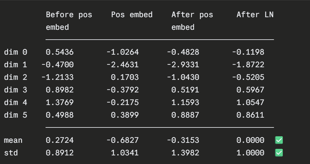
Figure 8: Layer Normalization
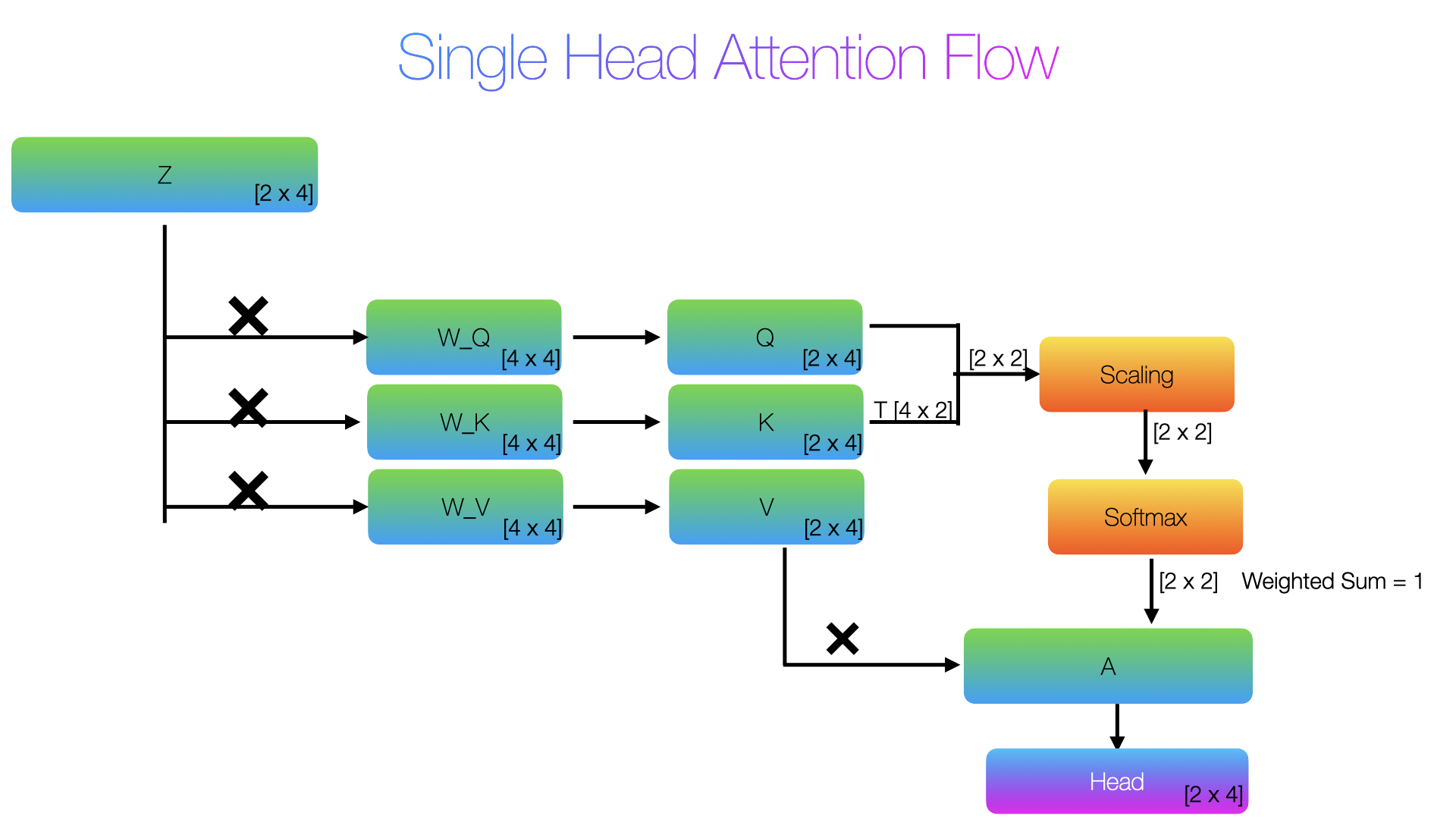
Self-Attention Mechanism for Single Head
After positional embedding and layer normalisation, each token is represented as a 768-dimensional vector. To understand clean math, let me simplify it for you with just four dimensions. In the original paper, it had 64 heads and 768 dimensions, but we will use 4 heads and 4 dimensions for easy understanding. Let’s say that we have the following CLS and one patch embedding tokens.
CLS    : [-0.1198, -1.8722, -0.5205, 0.5967]
patch1 : [0.4821, -0.9233, 0.7822, -0.3412]

# Make them into a tensor "Z"
Z = torch.tensor([
    [-0.1198, -1.8722, -0.5205,  0.5967],   # CLS   (position 0)
    [ 0.4821, -0.9234,  0.7823, -0.3412],   # patch1 (position 1)
], dtype=torch.float32)

# This is your input. 2 tokens, 4 dimensions each.
Self attention means the sequence attends to itself, every token in the sequence attends to every other token in the same sequence. The core mechanism is that every token produces 3 vector namely:
Q — Query "what am I looking for?"
K — Key "what do I contain?"
V — Value "what will I share if someone attends to me?"
Next is we have three Linear Projections or 3 randomly initialized weights created namely → W_Q, W_K and W_V
W_Q = torch.tensor([
    [0.1, 0.2, 0.3, 0.4],
    [0.5, 0.6, 0.7, 0.8],
    [0.2, 0.1, 0.4, 0.3],
    [0.6, 0.5, 0.8, 0.7],
], dtype=torch.float32)

W_K = torch.tensor([
    [0.3, 0.1, 0.4, 0.2],
    [0.7, 0.5, 0.8, 0.6],
    [0.1, 0.3, 0.2, 0.4],
    [0.5, 0.7, 0.6, 0.8],
], dtype=torch.float32)

W_V = torch.tensor([
    [0.4, 0.3, 0.2, 0.1],
    [0.8, 0.7, 0.6, 0.5],
    [0.3, 0.4, 0.1, 0.2],
    [0.7, 0.8, 0.5, 0.6],
], dtype=torch.float32)
In order to compute the Q, K, V we do matrix multiplication with Z with the respective initialized weights.
Z shape is [2, 4]
W_Q, W_K, W_V shape is [4, 4]

Q = Z * W_Q
# Q → shape becomes([2, 4])
  CLS    Q : [-0.694159984588623, -0.9009801149368286, -1.0773199796676636, -1.2841399908065796]
  patch1 Q : [-0.46174997091293335, -0.5499899983406067, -0.4617899954319, -0.550029993057251]


K = Z * W_K
# K → shape becomes([2, 4])
  CLS    K : [-1.1001800298690796, -0.6865400075912476, -1.291759967803955, -0.8781200647354126]
  patch1 K : [-0.5941200256347656, -0.41764000058174133, -0.5941399931907654, -0.4176599979400635]


V = Z * W_V
# V → shape becomes([2, 4])
  CLS    V : [-1.2841399908065796, -1.0773199796676636, -0.9009801149368286, -0.694159984588623]
  patch1 V : [-0.550029993057251, -0.4617899954319, -0.5499899983406067, -0.46174997091293335]
Compute Attention Score
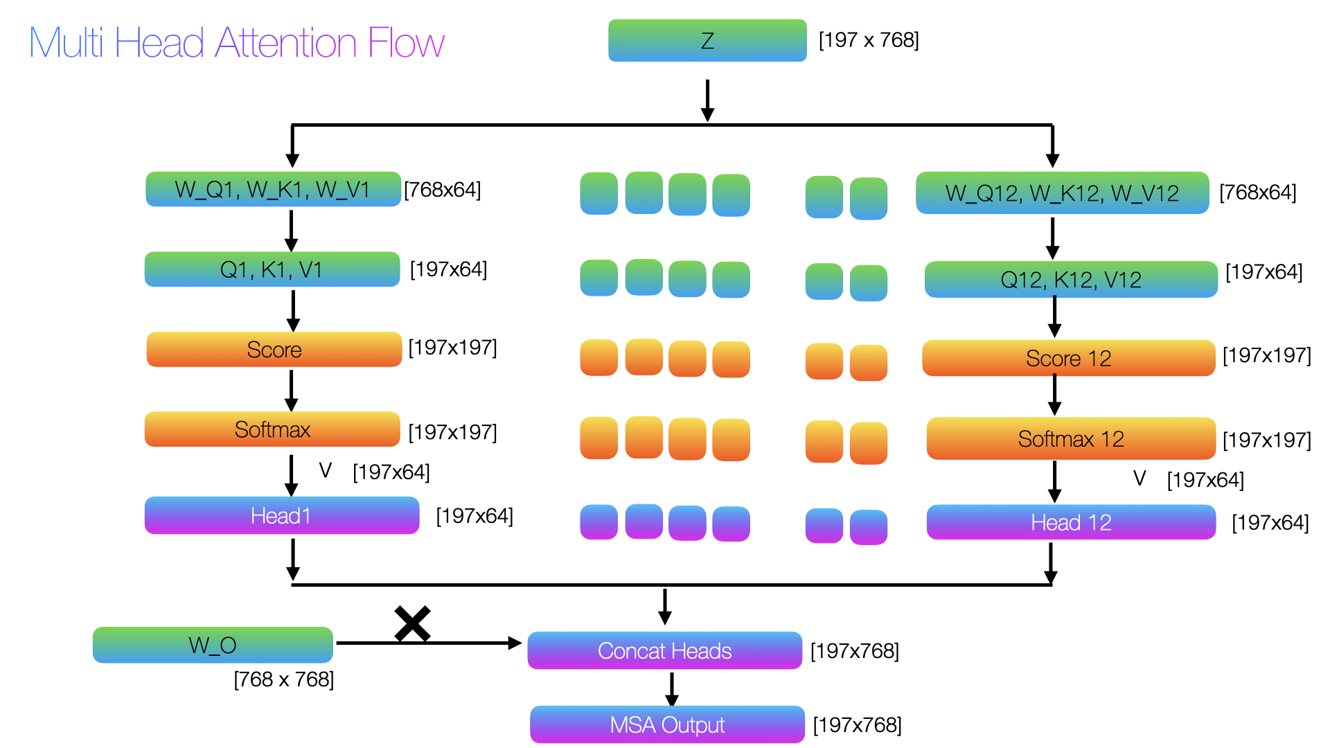
The paper computes attention as a softmax of matrix multiplication between Q and the transpose of K to the square root of the scale value. We need to know about scaling. While computing softmax, to prevent large values from killing the softmax gradient, we do scaling. In the ViT paper, the scale was set to 64 since the ViT base used 12 heads, so 768/12 = 64. But in our example data, we have 4 dimensions and the head is set to 4.
single head:   d_head = d_model / 1 = 4 / 1 = 4
two heads:     d_head = d_model / 2 = 4 / 2 = 2
twelve heads:  d_head = d_model / 12 = 768 / 12 = 64
Now lets get in to Attention calculation
Q = (Q . KT)/sqrt(scale)
A = softmax(Q)

# For our example value, we would get
Q = tensor([[1.9508, 0.9826],
        [0.9826, 0.5041]])

# Attention Matrix
A = tensor([[0.7248, 0.2752],
        [0.6174, 0.3826]])
Next we compute the weighted mix of values from attention and V matrix
Output = A . V

NEW_CLS = [-1.0820850133895874, -0.9079028367996216, -0.8043743371963501, -0.6301919221878052]
NEW_PATCH1 =[-1.0032637119293213, -0.841813325881958, -0.7666884660720825, -0.6052380204200745]
Quick Summary:
  INPUT  Z (after LayerNorm):
    CLS    : [-0.11980000138282776, -1.8722000122070312, -0.5205000042915344, 0.5967000126838684]
    patch1 : [0.4821000099182129, -0.9233999848365784, 0.7822999954223633, -0.34119999408721924]

  ATTENTION WEIGHTS (who attends to whom):
    CLS    → CLS    : 0.7248  (72.5%)
    CLS    → patch1 : 0.2752  (27.5%)
    patch1 → CLS    : 0.6174  (61.7%)
    patch1 → patch1 : 0.3826  (38.3%)

  OUTPUT (tokens enriched with context):
    new CLS    : [-1.0820850133895874, -0.9079028367996216, -0.8043743371963501, -0.6301919221878052]
    new patch1 : [-1.0032637119293213, -0.841813325881958, -0.7666884660720825, -0.6052380204200745]

  KEY TAKEAWAYS:
    old CLS knew only about itself
    new CLS    = 72.5% itself + 27.5% patch1
    old patch1 knew only about itself
    new patch1 = 61.7% CLS + 38.3% itself
Self-Attention Mechanism for Multi Head
Multi head attention is quite similar to single head attention, but now the number of head will change. Say if we have two heads, then
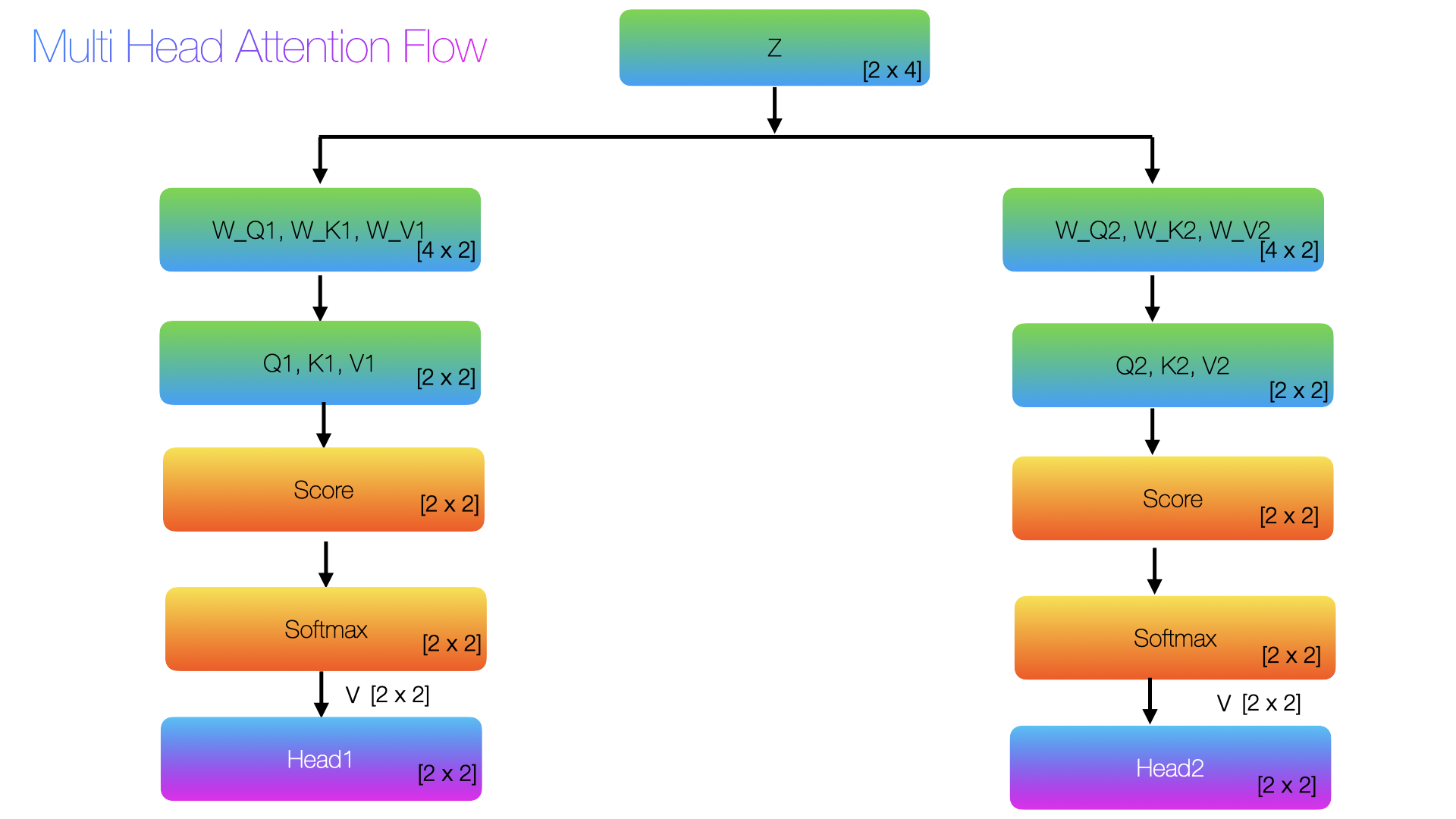
d_model   = 4
num_heads = 2
d_head    = d_model // num_heads    # 4 // 2 = 2

or in the original paper its 12 heads
d_head = d_model / 12 = 768 / 12 = 64


# Say if we have just two heads, then
# head 1 gets columns 0:2, head 2 gets columns 2:4
W_Q1, W_Q2 = W_Q[:, :d_head], W_Q[:, d_head:]   # [4×2], [4×2]
W_K1, W_K2 = W_K[:, :d_head], W_K[:, d_head:]   # [4×2], [4×2]
W_V1, W_V2 = W_V[:, :d_head], W_V[:, d_head:]   # [4×2], [4×2]
The rest of the calculation will be quite similar to single head. But in the multi head, we get d_head outputs. If we have 2 heads, we will get two head outputs
head1 = A1 @ V1

head1 [2×2]:
tensor([[-0.9930, -0.8332],
        [-0.9663, -0.8108]])

head2 = A2 @ V2

  head2 [2×2]:
tensor([[-0.8031, -0.6293],
        [-0.7607, -0.6013]])
Now, we will concatenate these head1 and head2 results
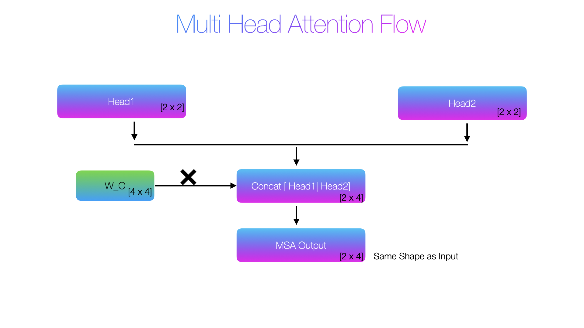
  concat [2×4] = [head1 | head2]:
  CLS    : [-0.9930022954940796, -0.8332093954086304] | [-0.8030619621276855, -0.6293230056762695]
         = [-0.9930022954940796, -0.8332093954086304, -0.8030619621276855, -0.6293230056762695]
  patch1 : [-0.966303825378418, -0.8108235597610474] | [-0.7607036232948303, -0.6012750864028931]
         = [-0.966303825378418, -0.8108235597610474, -0.7607036232948303, -0.6012750864028931]
Now there is a new matrix Wo, In this example its [4,4] matrix, the purpose is to mix all head outputs into one integrated representation
W_O = torch.tensor([
    [0.3, 0.1, 0.4, 0.2],
    [0.7, 0.5, 0.8, 0.6],
    [0.1, 0.3, 0.2, 0.4],
    [0.5, 0.7, 0.6, 0.8],
], dtype=torch.float32)


#[2,4] = [2,4] @ [4,4]
output = concat @ Wo

── Final MSA output ─────────────────────────────────────
  CLS    : [-1.2761149406433105, -1.1973495483398438, -1.601974606513977, -1.5232093334197998]
  patch1 : [-1.2341755628585815, -1.1511458158493042, -1.548086166381836, -1.4650564193725586]
Comparing with the original paper
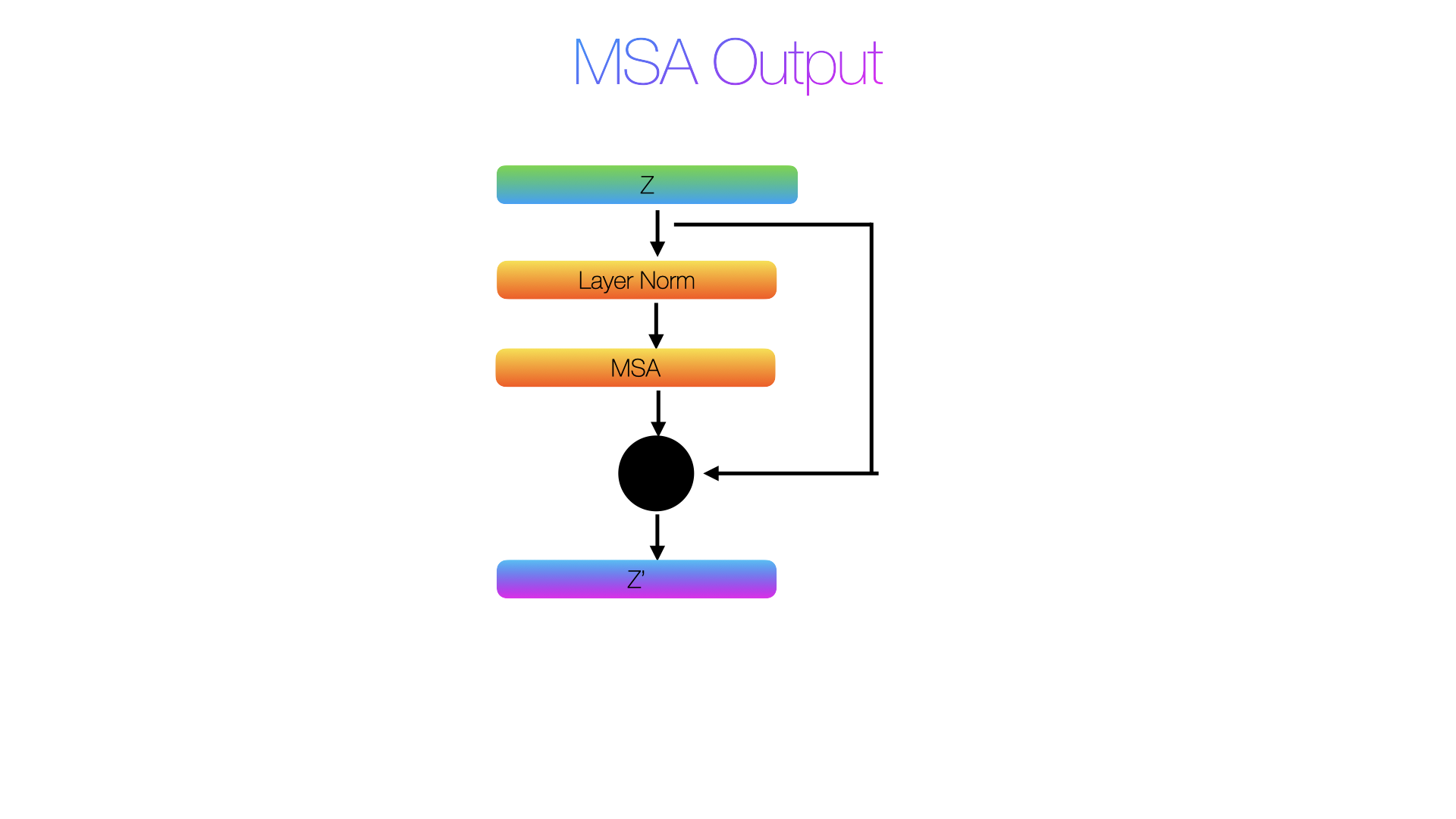
Skip Connection
It is the simplest operation in the entire Transformer and its just an addition:
z′= MSA(LN(z)) + z
The + z at the end is the skip connection. That is literally it. But why are they needed here?
Deep networks suffer from two problems:
Vanishing gradients: During backpropagation gradients flow backwards through every layer. Each layer multiplies the gradient by its weights. After 12 layers of multiplication the gradient can become extremely small, essentially zero. The early layers stop learning.
Degradation: Deeper networks should be at least as good as shallower ones, worst case a layer could just learn to pass input through unchanged (identity function). But without skip connections layers find it hard to learn identity, they always transform the input.
Using the actual values from our toy example:
CLS:
  dim0: -1.2761 + (-0.1198) = -1.3959
  dim1: -1.1973 + (-1.8722) = -3.0695
  dim2: -1.6020 + (-0.5205) = -2.1225
  dim3: -1.5232 + ( 0.5967) = -0.9265

patch1:
  dim0: -1.2342 + ( 0.4821) = -0.7521
  dim1: -1.1511 + (-0.9234) = -2.0745
  dim2: -1.5481 + ( 0.7823) = -0.7658
  dim3: -1.4651 + (-0.3412) = -1.8063
This is how a skip connection restores the differences between CLS and patch1 that attention had blurred.
CLS    z': [-1.3959, -3.0695, -2.1225, -0.9265]
patch1 z': [-0.7521, -2.0745, -0.7658, -1.8063]
MLP Layer
Just before the MLP, and after the MSA step, we have another layer normalisation, which does a similar step to the one we discussed previously. We will therefore proceed directly to the MLP layer next. The MLP layer consists of two linear layers and one GELU(non-linear activation). The order is linear layer which expands first, followed by a GELU activation and finally another linear layer with a compression. The expansion in the first linear layer provides wider thinking space and different combinations to explore. Then the GELU activation selects which combinations matter. Without the expansion, the MLP would be two linear layers, which collapse to a single linear transformation and no additional expressivity. The expansion with non-linearity in between is what gives the MLP its power. So, MSA gathers information from everywhere, and MLP processes that information deeply within each token.
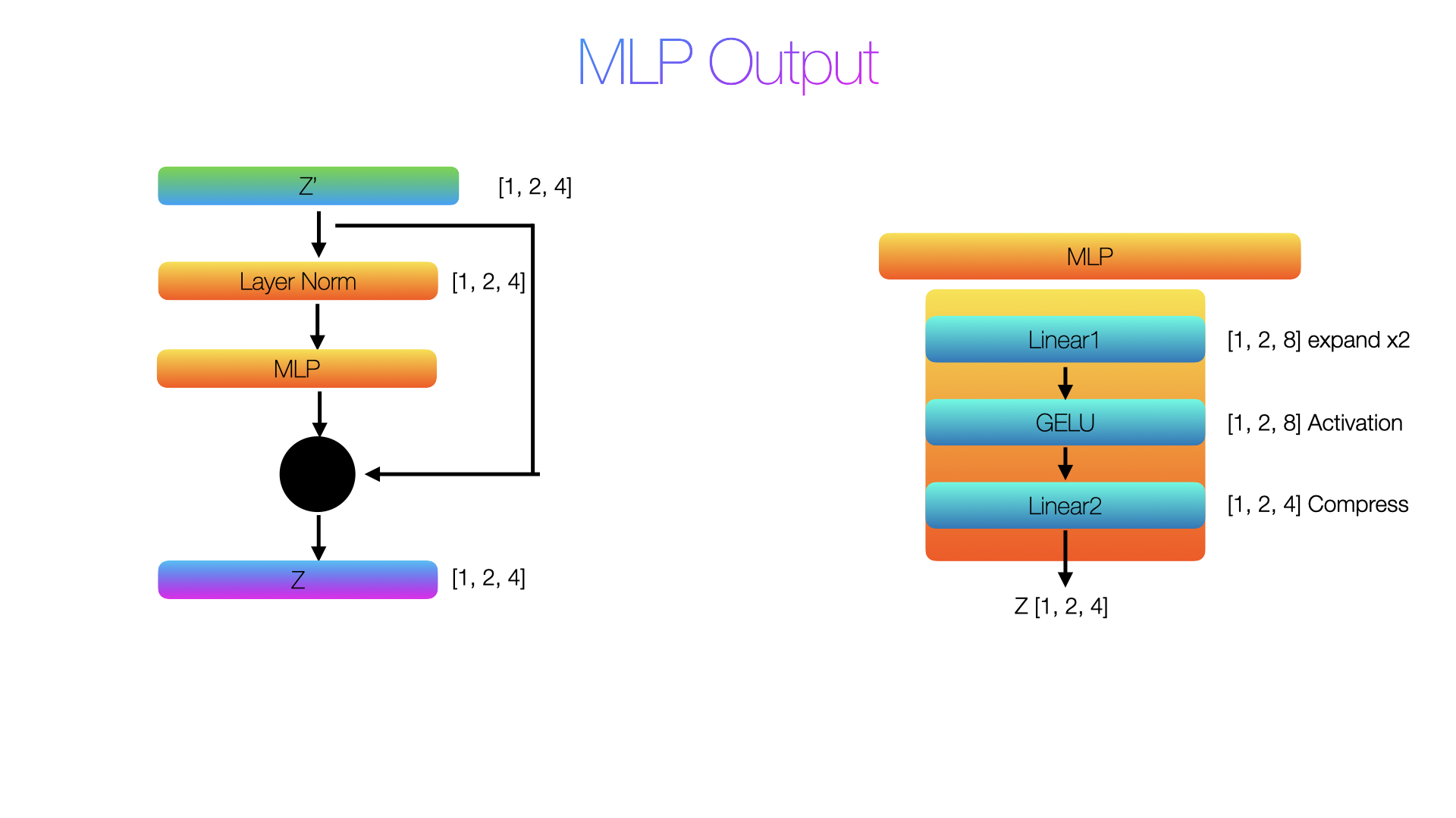
After Linear1 (expand 4 → 8):
  CLS    shape: torch.Size([1, 2, 8])  → [0.5790756940841675, 0.2883169949054718, 0.6198204755783081, 0.2739303708076477, 0.41952085494995117, 0.804477334022522, -0.15279024839401245, -0.03854984790086746]
  patch1 shape: torch.Size([1, 2, 8])  → [-0.1997881531715393, -0.6100909113883972, 1.074939489364624, 0.8850420713424683, 0.04830671846866608, -0.20638227462768555, 0.031368136405944824, 1.2525125741958618]

After GELU:
  CLS    : [0.4161996841430664, 0.17686745524406433, 0.453902006149292, 0.16653074324131012, 0.27796706557273865, 0.6350860595703125, -0.06711796671152115, -0.0186822060495615]
  patch1 : [-0.08407548069953918, -0.16527408361434937, 0.9231569766998291, 0.7185949087142944, 0.02508394792675972, -0.08631861954927444, 0.016076549887657166, 1.1207586526870728]

After Linear2 (compress 8 → 4):
  CLS    : [0.42665982246398926, -0.33748236298561096, -0.3735828995704651, -0.3624216318130493]
  patch1 : [0.8049083948135376, -0.5585855841636658, -0.39746788144111633, -0.003347724676132202]

After residual (MLP output + z'):
  CLS    : [-0.9692401885986328, -3.406982421875, -2.4960827827453613, -1.288921594619751]
  patch1 : [0.052808403968811035, -2.6330857276916504, -1.1632678508758545, -1.809647798538208]
This becomes the entire Transformer encoder block, in our example input shape is shape was (1, 2, 4) and finally the output shape is also (1, 2, 4). This block is repeated for N blocks and the output will be same (1, 2, 4).
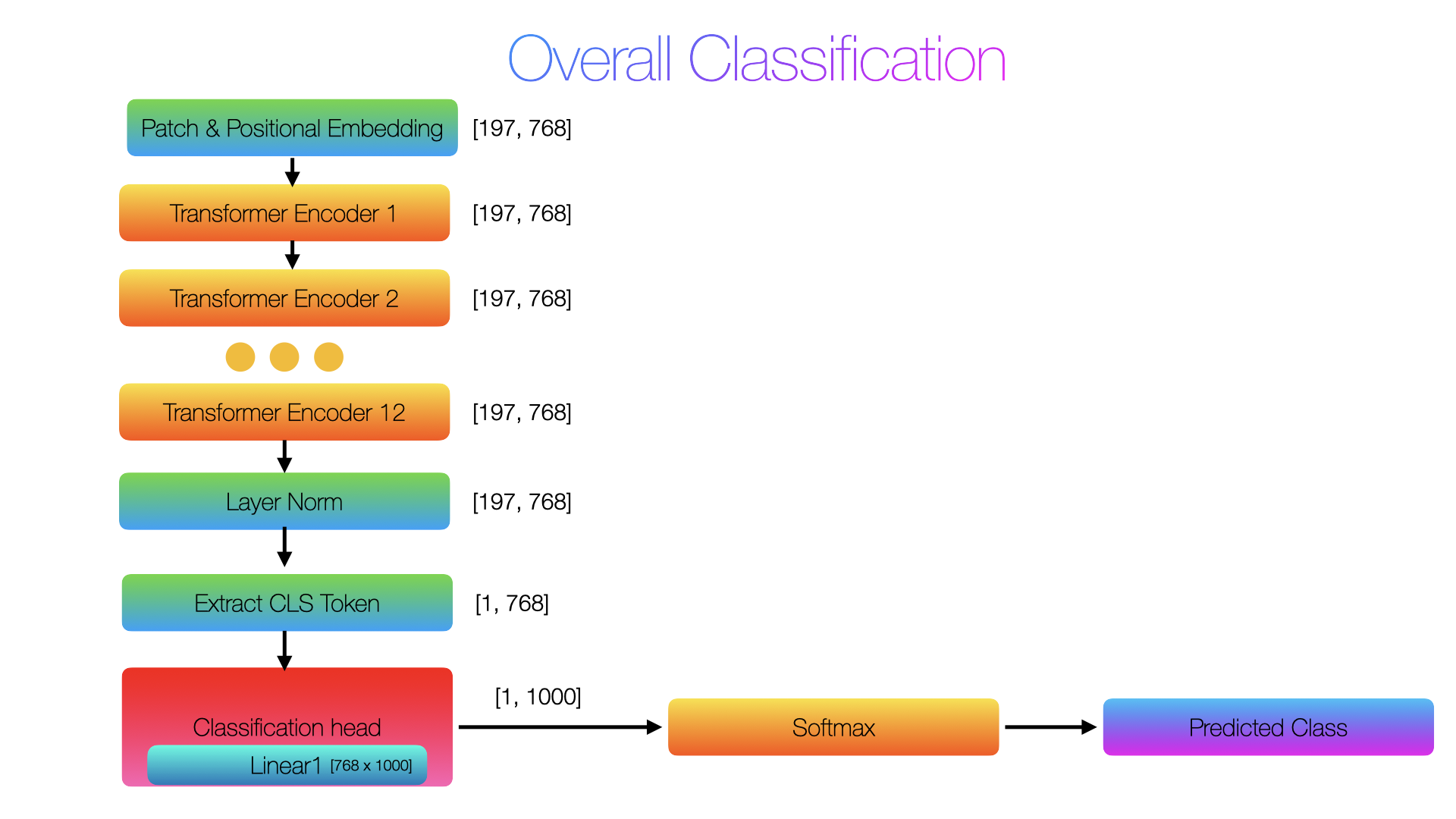
MLP Head
This is the final step before final classification, in this step we will do layer normalization, then extract CLS token class then pass it to a linear layer and at the end convert to probabilities for the class.
 Thiyaga Bot